Training Multi-Layer RNN with Constrained Weights#

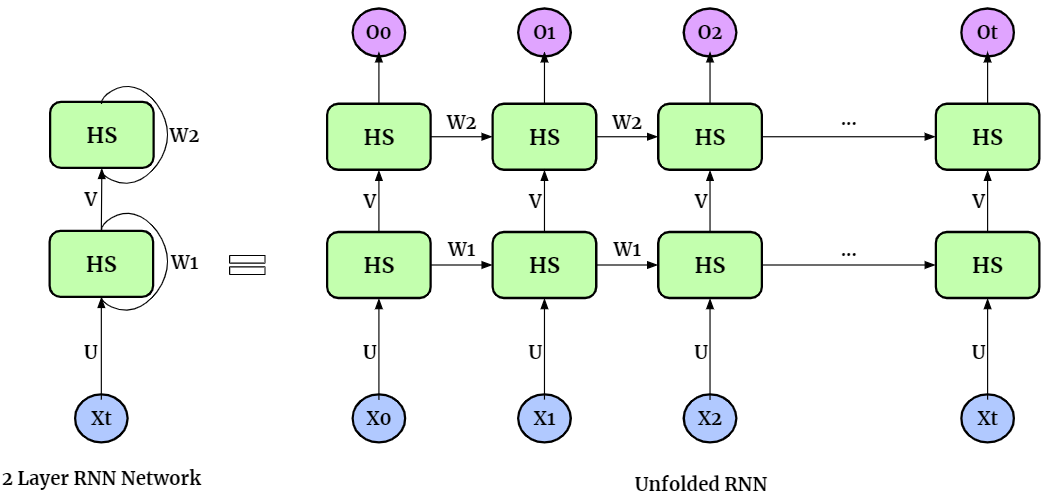
The multi-layer RNN are developed to create higher-level abstractions and capture more non-linearities between the data. With N_layer layers, multi-layer RNN has N_layer hidden states. Here is an example for two-layer RNN,

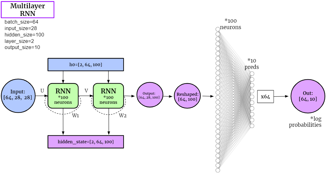
Similar to single-layer cases, when applied to the classification tasks on MNIST dataset, the structure of multi-layer RNN can be expressed as

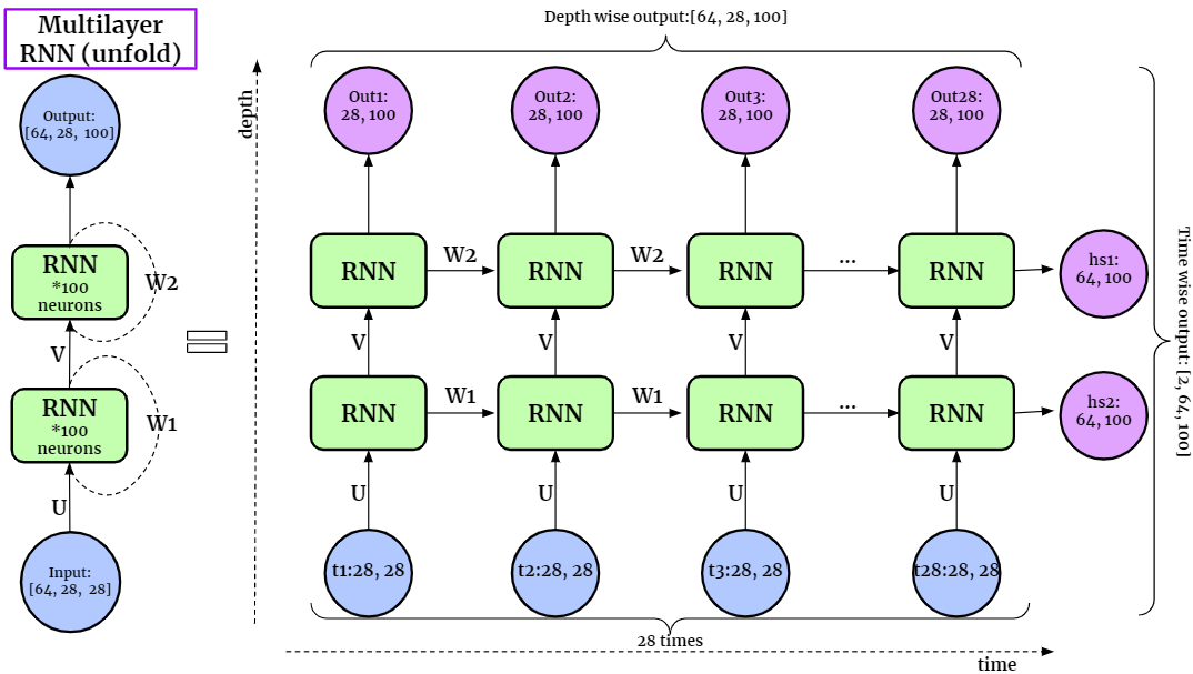
If we unfold the Multilayer RNN layer, it can be expressed as

Import modules#

# Imports
import torch
import torch.nn as nn
import torch.nn.functional as F
import torch.optim as optim
import os
import numpy as np

import torchvision
import torchvision.transforms as transforms

import matplotlib.pyplot as plt
%matplotlib inline
import sklearn.metrics
import seaborn as sns
import random

from torch.nn.parameter import Parameter

# To display youtube videos
from IPython.display import YouTubeVideo
from cdopt.manifold_torch import euclidean_torch, stiefel_torch
from cdopt.nn import RNN_cdopt, get_quad_penalty


def set_seed(seed = 1234):
    '''Sets the seed of the entire notebook so results are the same every time we run.
    This is for REPRODUCIBILITY.'''
    np.random.seed(seed)
    random.seed(seed)
    torch.manual_seed(seed)
    torch.cuda.manual_seed(seed)
    # When running on the CuDNN backend, two further options must be set
    torch.backends.cudnn.deterministic = True
    # Set a fixed value for the hash seed
    os.environ['PYTHONHASHSEED'] = str(seed)
    
set_seed()

device = torch.device('cuda' if torch.cuda.is_available() else 'cpu')
print('Device available now:', device)

Device available now: cuda

Define the network#

Define a neurnal with constrained weights are quite simple via CDOpt, we only need the following two procedures:

Replace the layers in torch.nn by the layers from cdopt.utils_torch.nn and specify the manifold_class options.
Add the layer.quad_penalty() to the loss function.

class MultilayerRNN_MNIST(nn.Module):
    def __init__(self, input_size, hidden_size, layer_size, output_size, relu=True):
        super(MultilayerRNN_MNIST, self).__init__()
        self.input_size, self.hidden_size, self.layer_size, self.output_size = input_size, hidden_size, layer_size, output_size
        
        # Create RNN. Users can try other manifold classes from `cdopt.manifold_torch` in the setup of `cdopt.nn.RNN_cdopt`. 
        if relu:
            self.rnn = RNN_cdopt(input_size, hidden_size, layer_size, batch_first=True, nonlinearity='relu', manifold_class = stiefel_torch, penalty_param = 0.2)
        else:
            self.rnn = RNN_cdopt(input_size, hidden_size, layer_size, batch_first=True, nonlinearity='tanh', manifold_class = stiefel_torch, penalty_param = 0.2)
            
        # Create FNN
        self.fnn = nn.Linear(hidden_size, output_size)
        
    def forward(self, images, prints=False):
        if prints: print('images shape:', images.shape)
        
        # Instantiate hidden_state at timestamp 0
        hidden_state = torch.zeros(self.layer_size, images.size(0), self.hidden_size).to(device)
        hidden_state = hidden_state.requires_grad_()
        if prints: print('Hidden State shape:', hidden_state.shape)
        
        # Compute RNN
        # .detach() is required to prevent vanishing gradient problem
        output, last_hidden_state = self.rnn(images, hidden_state.detach())
        if prints: print('RNN Output shape:', output.shape, '\n' +
                         'RNN last_hidden_state shape', last_hidden_state.shape)
        
        # Compute FNN
        # We get rid of the second size
        output = self.fnn(output[:, -1, :])
        if prints: print('FNN Output shape:', output.shape)
        
        return output

Training RNN#

We’ll use get_accuracy() and train_network() functions from the examples on Kaggle, but with some changes (suited to the RNN’s needs).

# Customized transform (transforms to tensor, here you can normalize, perform Data Augmentation etc.)
my_transform = transforms.Compose([transforms.ToTensor()])

# Download data
mnist_train = torchvision.datasets.MNIST('data', train = True, download=True, transform=my_transform)
mnist_test = torchvision.datasets.MNIST('data', train = False, download=True, transform=my_transform)

def get_accuracy(out, actual_labels, batchSize):
    '''Saves the Accuracy of the batch.
    Takes in the log probabilities, actual label and the batchSize (to average the score).'''
    predictions = out.max(dim=1)[1]
    correct = (predictions == actual_labels).sum().item()
    accuracy = correct/batch_size
    
    return accuracy

def train_network(model, train_data, test_data, batchSize=64, num_epochs=1, learning_rate=0.0005):
    
    '''Trains the model and computes the average accuracy for train and test data.'''
    
    print('Get data ready...')
    # Create dataloader for training dataset - so we can train on multiple batches
    # Shuffle after every epoch
    train_loader = torch.utils.data.DataLoader(dataset=train_data, batch_size=batchSize, shuffle=True, drop_last=True)
    test_loader = torch.utils.data.DataLoader(dataset=test_data, batch_size=batchSize, shuffle=True, drop_last=True)
    
    # Create criterion and optimizer
    criterion = nn.CrossEntropyLoss()
    optimizer = optim.Adam(model.parameters(), lr=learning_rate)
    
    
    print('Training started...')
    # Train the data multiple times
    for epoch in range(num_epochs):
        
        # Save Train and Test Loss
        train_loss = 0
        train_acc = 0

        
        # Set model in training mode:
        model.train()

        
        
        for k, (images, labels) in enumerate(train_loader):
            
            # Get rid of the channel
            images = images.view(-1, 28, 28)
            images = images.to(device)
            labels = labels.to(device)
            # print(labels.device)
            # Create log probabilities
            out = model(images)
            # Clears the gradients from previous iteration
            optimizer.zero_grad()
            # Computes loss: how far is the prediction from the actual?
            loss = criterion(out, labels) + get_quad_penalty(model)
            # Computes gradients for neurons
            loss.backward()
            # Updates the weights
            optimizer.step()
            
            # Save Loss & Accuracy after each iteration
            train_loss += loss.item()
            train_acc += get_accuracy(out, labels, batchSize)
            
        
        # Print Average Train Loss & Accuracy after each epoch
        print('TRAIN | Epoch: {}/{} | Loss: {:.2f} | Accuracy: {:.2f}'.format(epoch+1, num_epochs, train_loss/k, train_acc/k))
            
            
    print('Testing Started...')
    # Save Test Accuracy
    test_acc = 0
    # Evaluation mode
    model.eval()
    
    for k, (images, labels) in enumerate(test_loader):
        # Get rid of the channel
        images = images.view(-1, 28, 28)
        images = images.to(device)
        labels = labels.to(device)
        # Create logit predictions
        out = model(images)
        # Add Accuracy of this batch
        test_acc += get_accuracy(out, labels, batchSize)
        
    # Print Final Test Accuracy
    print('TEST | Average Accuracy per {} Loaders: {:.5f}'.format(k, test_acc/k) )

# ==== STATICS ====
batch_size = 64
input_size = 28
hidden_size = 100  
layer_size = 2         
output_size = 10

# Instantiate the model
# We'll use TANH as our activation function
multilayer_rnn = MultilayerRNN_MNIST(input_size, hidden_size, layer_size, output_size, relu=False)
multilayer_rnn.to(device)
# ==== TRAIN ====
train_network(multilayer_rnn, mnist_train, mnist_test, num_epochs=10)

Get data ready...
Training started...
TRAIN | Epoch: 1/10 | Loss: 0.56 | Accuracy: 0.85
TRAIN | Epoch: 2/10 | Loss: 0.24 | Accuracy: 0.93
TRAIN | Epoch: 3/10 | Loss: 0.19 | Accuracy: 0.95
TRAIN | Epoch: 4/10 | Loss: 0.16 | Accuracy: 0.95
TRAIN | Epoch: 5/10 | Loss: 0.14 | Accuracy: 0.96
TRAIN | Epoch: 6/10 | Loss: 0.13 | Accuracy: 0.96
TRAIN | Epoch: 7/10 | Loss: 0.12 | Accuracy: 0.96
TRAIN | Epoch: 8/10 | Loss: 0.12 | Accuracy: 0.96
TRAIN | Epoch: 9/10 | Loss: 0.11 | Accuracy: 0.97
TRAIN | Epoch: 10/10 | Loss: 0.11 | Accuracy: 0.97
Testing Started...
TEST | Average Accuracy per 155 Loaders: 0.97016

multilayer_rnn.rnn.quad_penalty()

tensor(0.0024, device='cuda:0', grad_fn=<AddBackward0>)

Reference#

https://www.kaggle.com/code/andradaolteanu/pytorch-rnns-and-lstms-explained-acc-0-99
Jing L, Gulcehre C, Peurifoy J, et al. Gated orthogonal recurrent units: On learning to forget[J]. Neural computation, 2019, 31(4): 765-783.
Hu X, Xiao N, Liu X, Toh KC. A Constraint Dissolving Approach for Nonsmooth Optimization over the Stiefel Manifold[J]. arXiv preprint arXiv:2205.10500, 2022.

Constraint Dissolving Approaches for Riemannian Optimization

Training Multi-Layer RNN with Constrained Weights

Contents

Training Multi-Layer RNN with Constrained Weights#

Import modules#

Define the network#

Training RNN#

Reference#