Training Single-Layer RNN with Constrained Weights#

Recurrent Neural Networks are very different from FNNs or CNNs.

RNNs model sequential data, meaning they have sequential memory. An RNN takes in different kind of inputs (text, words, letters, parts of an image, sounds, etc.) and returns different kinds of outputs (the next word/letter in the sequence, paired with an FNN it can return a classification etc.). Here is an example for a RNN with 1 layer.

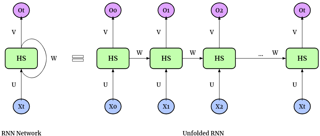
How RNN works:

It uses previous information to affect later ones
There are 3 layers: Input, Output and Hidden (where the information is stored)
The loop: passes the input forward sequentialy, while retaining information about it
This info is stored in the hidden state
There are only 3 matrixes (U, V, W) that contain weights as parameters. These DON’T change with the input, they stay the same through the entire sequence.

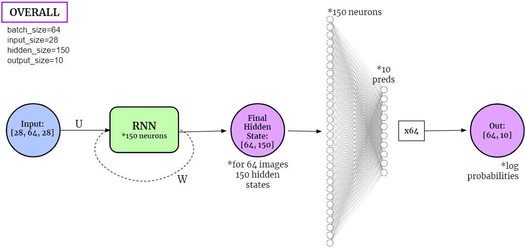
When applied to the classification tasks on MNIST dataset, the structure of the neural network becomes

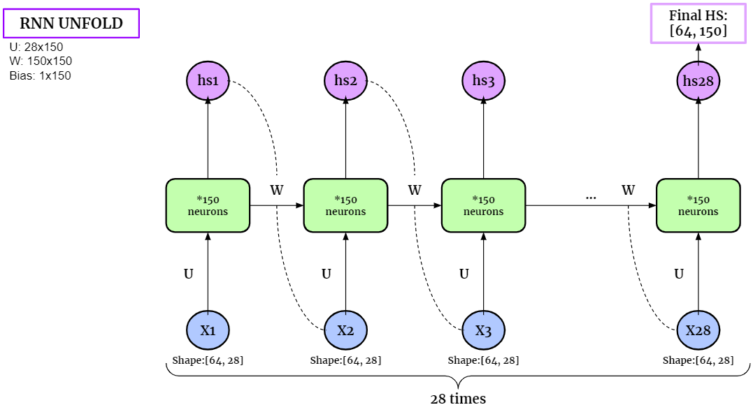
If we unfold the RNN layers, it becomes

# Imports
import torch
import torch.nn as nn
import torch.nn.functional as F
import torch.optim as optim
import os
import numpy as np

import torchvision
import torchvision.transforms as transforms

import matplotlib.pyplot as plt
%matplotlib inline
import sklearn.metrics
import seaborn as sns
import random

from torch.nn.parameter import Parameter

# To display youtube videos
from IPython.display import YouTubeVideo
import cdopt
from cdopt.manifold_torch import euclidean_torch, stiefel_torch
from cdopt.nn import RNN_cdopt, get_quad_penalty



def set_seed(seed = 1234):
    '''Sets the seed of the entire notebook so results are the same every time we run.
    This is for REPRODUCIBILITY.'''
    np.random.seed(seed)
    random.seed(seed)
    torch.manual_seed(seed)
    torch.cuda.manual_seed(seed)
    # When running on the CuDNN backend, two further options must be set
    torch.backends.cudnn.deterministic = True
    # Set a fixed value for the hash seed
    os.environ['PYTHONHASHSEED'] = str(seed)
    
set_seed()

device = torch.device('cuda' if torch.cuda.is_available() else 'cpu')
# device = torch.device('cpu')
print('Device available now:', device)

Device available now: cuda

Define the network#

Define a neurnal with constrained weights are quite simple via CDOpt, we only need the following two procedures:

Replace the layers in torch.nn by the layers from cdopt.utils_torch.nn and specify the manifold_class options.
Add the layer.quad_penalty() to the loss function.

# The Neural Network
class VanillaRNN_MNIST(nn.Module):
    def __init__(self, batch_size, input_size, hidden_size, output_size):
        super(VanillaRNN_MNIST, self).__init__()
        self.batch_size, self.input_size, self.hidden_size, self.output_size = batch_size, input_size, hidden_size, output_size
        
        # replace nn.RNN Layer by the layers from `cdopt.nn.RNN_cdopt`. Users can try other manifold classes from `cdopt.manifold_torch`
        self.rnn = RNN_cdopt(input_size, hidden_size, manifold_class = stiefel_torch, penalty_param = 0.2)
        # Fully Connected Layer. Users can try other manifold classes from `cdopt.manifold_torch`.
        self.layer = nn.Linear(hidden_size, self.output_size)
        # self.layer = cdopt.nn.Linear_cdopt(hidden_size, self.output_size, manifold_class= stiefel_torch)
    
    def forward(self, images, prints=False):
        if prints: print('Original Images Shape:', images.shape)
        
        images = images.permute(1, 0, 2)
        if prints: print('Permuted Imaged Shape:', images.shape)
        
        # Initialize hidden state with zeros
        hidden_state = torch.zeros(1, self.batch_size, self.hidden_size, device = device)
        if prints: print('Initial hidden state Shape:', hidden_state.shape)
        
        # Creating RNN
        hidden_outputs, hidden_state = self.rnn(images, hidden_state)
        
        # Log probabilities
        out = self.layer(hidden_state)
        
        if prints:
            print('----hidden_outputs shape:', hidden_outputs.shape, '\n' +
                  '----final hidden state:', hidden_state.shape, '\n' +
                  '----out shape:', out.shape)
        
        # Reshaped out
        out = out.view(-1, self.output_size)
        if prints: print('Out Final Shape:', out.shape)
        
        return out

Training RNN#

We’ll use get_accuracy() and train_network() functions from the examples on Kaggle, but with some changes (suited to the RNN’s needs).

# Customized transform (transforms to tensor, here you can normalize, perform Data Augmentation etc.)
my_transform = transforms.Compose([transforms.ToTensor()])

# Download data
mnist_train = torchvision.datasets.MNIST('data', train = True, download=True, transform=my_transform)
mnist_test = torchvision.datasets.MNIST('data', train = False, download=True, transform=my_transform)

def get_accuracy(out, actual_labels, batchSize):
    '''Saves the Accuracy of the batch.
    Takes in the log probabilities, actual label and the batchSize (to average the score).'''
    predictions = out.max(dim=1)[1]
    correct = (predictions == actual_labels).sum().item()
    accuracy = correct/batch_size
    
    return accuracy

def train_network(model, train_data, test_data, batchSize=64, num_epochs=1, learning_rate=0.0005):
    
    '''Trains the model and computes the average accuracy for train and test data.'''
    
    print('Get data ready...')
    # Create dataloader for training dataset - so we can train on multiple batches
    # Shuffle after every epoch
    train_loader = torch.utils.data.DataLoader(dataset=train_data, batch_size=batchSize, shuffle=True, drop_last=True)
    test_loader = torch.utils.data.DataLoader(dataset=test_data, batch_size=batchSize, shuffle=True, drop_last=True)
    
    # Create criterion and optimizer
    criterion = nn.CrossEntropyLoss()
    optimizer = optim.Adam(model.parameters(), lr=learning_rate)
    
    
    print('Training started...')
    # Train the data multiple times
    for epoch in range(num_epochs):
        
        # Save Train and Test Loss
        train_loss = 0
        train_acc = 0

        
        # Set model in training mode:
        model.train()

        
        
        for k, (images, labels) in enumerate(train_loader):
            
            # Get rid of the channel
            images = images.view(-1, 28, 28)
            images = images.to(device)
            labels = labels.to(device)
            # print(labels.device)
            # Create log probabilities
            out = model(images)
            # Clears the gradients from previous iteration
            optimizer.zero_grad()
            # Computes loss: how far is the prediction from the actual? And add the layer.quad_penalty() to the loss function. 
            loss = criterion(out, labels) + get_quad_penalty(model)
            # Computes gradients for neurons
            loss.backward()
            # Updates the weights
            optimizer.step()
            
            # Save Loss & Accuracy after each iteration
            train_loss += loss.item()
            train_acc += get_accuracy(out, labels, batchSize)
            
        
        # Print Average Train Loss & Accuracy after each epoch
        print('TRAIN | Epoch: {}/{} | Loss: {:.2f} | Accuracy: {:.2f}'.format(epoch+1, num_epochs, train_loss/k, train_acc/k))
            
            
    print('Testing Started...')
    # Save Test Accuracy
    test_acc = 0
    # Evaluation mode
    model.eval()
    
    for k, (images, labels) in enumerate(test_loader):
        # Get rid of the channel
        images = images.view(-1, 28, 28)
        images = images.to(device)
        labels = labels.to(device)
        # Create logit predictions
        out = model(images)
        # Add Accuracy of this batch
        test_acc += get_accuracy(out, labels, batchSize)
        
    # Print Final Test Accuracy
    print('TEST | Average Accuracy per {} Loaders: {:.5f}'.format(k, test_acc/k) )

# ==== STATICS ====
batch_size=64
input_size=28
hidden_size=150
output_size=10

# Instantiate the model
vanilla_rnn = VanillaRNN_MNIST(batch_size, input_size, hidden_size, output_size)

vanilla_rnn.to(device)

VanillaRNN_MNIST(
  (rnn): RNN_cdopt(28, 150)
  (layer): Linear(in_features=150, out_features=10, bias=True)
)

# ==== TRAIN ====
train_network(vanilla_rnn, mnist_train, mnist_test, num_epochs=10)

Get data ready...
Training started...
TRAIN | Epoch: 1/10 | Loss: 0.86 | Accuracy: 0.79
TRAIN | Epoch: 2/10 | Loss: 0.41 | Accuracy: 0.89
TRAIN | Epoch: 3/10 | Loss: 0.30 | Accuracy: 0.92
TRAIN | Epoch: 4/10 | Loss: 0.25 | Accuracy: 0.93
TRAIN | Epoch: 5/10 | Loss: 0.22 | Accuracy: 0.94
TRAIN | Epoch: 6/10 | Loss: 0.20 | Accuracy: 0.95
TRAIN | Epoch: 7/10 | Loss: 0.18 | Accuracy: 0.95
TRAIN | Epoch: 8/10 | Loss: 0.17 | Accuracy: 0.95
TRAIN | Epoch: 9/10 | Loss: 0.15 | Accuracy: 0.96
TRAIN | Epoch: 10/10 | Loss: 0.15 | Accuracy: 0.96
Testing Started...
TEST | Average Accuracy per 155 Loaders: 0.96522

vanilla_rnn.rnn.quad_penalty()

tensor(0.0035, device='cuda:0', grad_fn=<AddBackward0>)

Reference#

https://www.kaggle.com/code/andradaolteanu/pytorch-rnns-and-lstms-explained-acc-0-99
Jing L, Gulcehre C, Peurifoy J, et al. Gated orthogonal recurrent units: On learning to forget[J]. Neural computation, 2019, 31(4): 765-783.
Hu X, Xiao N, Liu X, Toh KC. A Constraint Dissolving Approach for Nonsmooth Optimization over the Stiefel Manifold[J]. arXiv preprint arXiv:2205.10500, 2022.

Constraint Dissolving Approaches for Riemannian Optimization

Training Single-Layer RNN with Constrained Weights

Contents

Training Single-Layer RNN with Constrained Weights#

Define the network#

Training RNN#

Reference#